---

Ever wondered how your phone can recognize your face or how Netflix seems to know exactly what movie you want to watch next? The magic behind much of this technology is a concept called a deep neural network.

At its core, a neural network is a powerful way for computers to learn from data. Think of it as a layered system that tries to find patterns, much like our own brains. The term “deep” simply means the network has multiple layers. In this post, we’ll break down the fundamental building blocks of these networks, from the data they eat to the “secret sauce” that lets them learn.

🧠 What is a Neural Network?

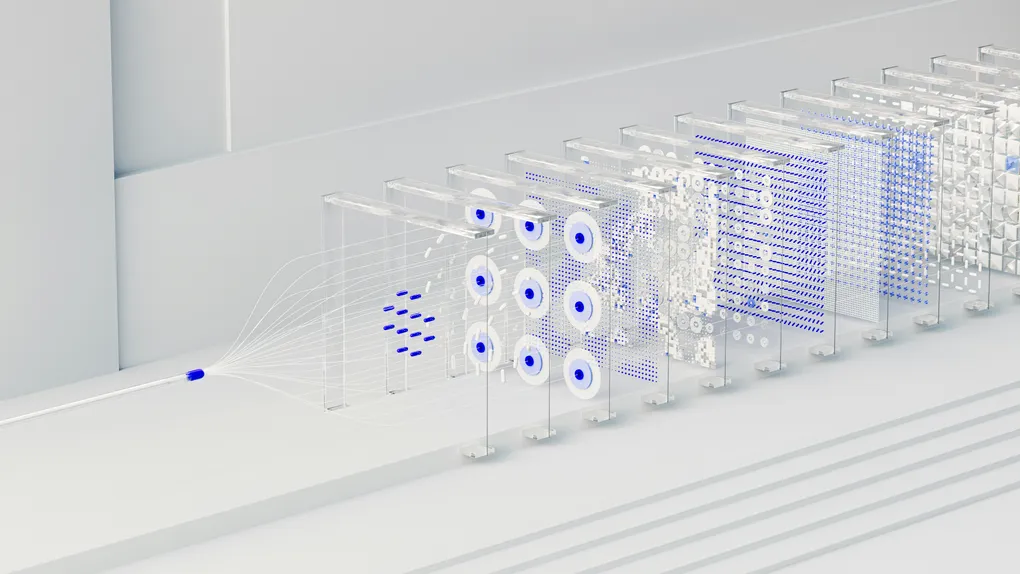
A neural network processes data by passing it through a series of layers. At each layer, it applies specific mathematical operations to transform the data, essentially looking at it from a new perspective. The goal is to learn more about the data at each step. By the time the data reaches the final layer, the network has a sophisticated understanding of it, allowing it to make an accurate prediction.

🧱 The Building Blocks: Data, Layers, and Neurons

Before a network can learn, it needs a solid structure. Let’s look at its core components.

1. Data: (The Fuel for the Network) A neural network can process many types of data, but it needs to be in a specific shape. Some of the most common data structures include:

   • Vector Data (2D): Think of rows in a spreadsheet, like customer information.

   • Timeseries or Sequence (3D): Data where order matters, like stock prices over time or words in a sentence.

   • Image Data (4D): A grid of pixels with color channels (height, width, color).

   • Video Data (5D): A sequence of images (frames, height, width, color).

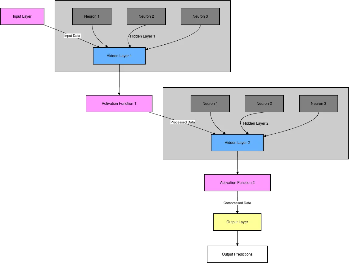
2. Layers: (The Assembly Line) Each network is made up of layers, and each layer has a specific job.

   • Input Layer: This is the front door of the network. Your initial data (like the pixels of an image) is fed into this layer.

   • Hidden Layers: These are the workhorse layers between the input and output. A network can have one or many hidden layers. The more complex the problem, the more hidden layers you’ll typically need. They’re called “hidden” simply because we don’t directly see their output.

   • Output Layer: This is the final layer where you get the result. It could be a single value (like the price of a house) or multiple values (like the probability of an image being a cat, dog, or bird).

3. Neurons: (The Individual Workers) Each layer is made up of neurons. A neuron is a tiny unit that holds a single numeric value. The input layer will have as many neurons as there are input data points. For example, a 28x28 pixel image has 784 pixels, so the input layer would need 784 neurons. The output layer will have as many neurons as there are required outputs. The number of neurons in a hidden layer is a design choice you make when building the network. When every neuron in one layer connects to every neuron in the next, it’s called a dense layer.

4. Activation Function: An activation function is a mathematical formula that takes an input value and transforms it into a specific, required output. It acts like a filter or a reshaping tool, changing the input into a more useful format based on a predefined rule. Different formulas are used depending on the desired outcome.

   • Sigmoid: This function takes any number and squishes it into a range between 0 and 1. This is useful for representing a probability.
   • ReLU (Rectified Linear Unit): This function’s rule is simple: if the input is positive, it leaves it unchanged; if it’s negative or zero, it makes it zero.
   • Tanh (Hyperbolic Tangent): This is similar to Sigmoid but maps any input into a range between -1 and 1.
   • Softmax: This function takes a list of numbers and converts them into a probability distribution, where each output is between 0 and 1, and the entire list sums up to 1.

⚙️ How It Works: The Math Behind the Magic

So, how does data actually get transformed as it moves through the network? It’s all about a few key mathematical concepts.

Weights and Biases: (The Control Knobs)

• Weights: Every connection between neurons has a weight, which is just a number. This weight represents the strength or importance of that connection. A higher weight means the signal from that neuron is amplified.

• Biases: Each layer also has a bias, which is a single constant value added to the results. A bias allows the network to shift the output up or down, giving it more flexibility—much like the y-intercept in the equation of a line.

Initially, all weights and biases are set to random values. The process of training is all about the network figuring out the optimal values for these “control knobs” to make the best predictions.

The Core Calculation: (Weighted Sum)

The value of any given neuron is calculated by taking a weighted sum of the values from all the neurons connected to it from the previous layer, and then adding the bias. The formula looks like this:

$$Y = \left( \sum_{i=0}^{n} w_{i} x_{i} \right) + b$$

Where:

• Y is the output of the current neuron.
• n is the number of connections.
• $w_i$ is the weight of each connection.
• $x_i$ is the value of each connected neuron from the previous layer.
• b is the bias for the layer.

The Secret Ingredient: (The Activation Function) There’s one crucial part missing from the equation above. If we only used weighted sums, the network could only learn simple, linear relationships. To learn complex patterns, we need to introduce non-linearity.

We do this by applying an activation function to our weighted sum. This function transforms the output and allows the network to model far more complex data.

The final equation for a neuron’s output is:

$$Y = F\!\left( \sum_{i=0}^{n} w_{i} x_{i} + b \right)$$

Where $F(x)$ is the activation function. Common activation functions include ReLU, Tanh, and Sigmoid.

🎓 The Learning Process: How a Network Gets Smart

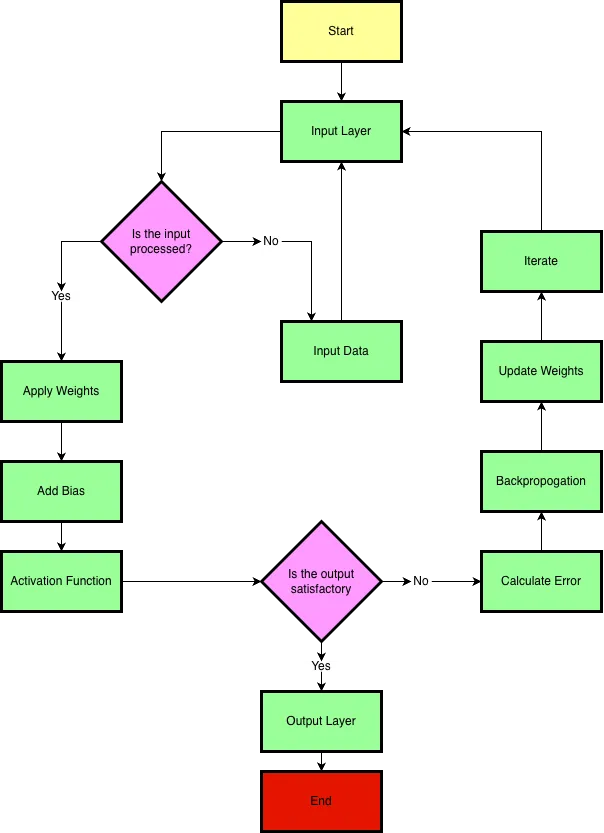
A brand-new network with random weights and biases is useless. It needs to be trained on data. Here’s how it learns from its mistakes.

1. The Loss/Cost Function (Grading the Test)

First, we need a way to measure how wrong our network’s predictions are. We feed the network some training data (for which we already know the correct answers) and compare its output to the actual labels.

A loss function (or cost function) calculates a score based on the difference between the predicted output and the expected output. A high score means the network did a poor job; a low score means it did well. The entire goal of training is to minimize this loss score.

2. Backpropagation & The Optimizer (Studying for the Retake)

Once we know how wrong the network is, we need to adjust its weights and biases to do better next time. This is where backpropagation comes in. It’s a clever algorithm that works backward from the loss score, figuring out how much each weight and bias contributed to the error.

An optimizer is the algorithm that implements this process. It uses a technique like Gradient Descent, which can be thought of as finding the quickest way down a hill. The “hill” is the loss function, and the optimizer iteratively tweaks the weights and biases to move in the direction that lowers the loss score the most.

Popular optimizers you’ll see include Stochastic Gradient Descent (SGD), Momentum, and Adam.

Conclusion

And that’s the core of it! A neural network is a system of interconnected layers of neurons that learns by: Passing data forward and making a prediction. Measuring how wrong its prediction was using a loss function. Adjusting its internal weights and biases using an optimizer to make a better prediction next time.

By repeating this process thousands of times, the network slowly tunes itself to become a powerful pattern-finding machine. Now that you understand the theory, you’re ready to start building your own with Keras!